This week I will give a brief introduction to piping and data wrangling with tidyr and tidyverse verbs. If you want to learn more, there are many resources on the web. I like this course book as a beginning, this course goes into more depth, and R for Data Science has much more.

Today’s goal is to teach you 6 data “verbs” that are easy to use and that will cover many of your data-wrangling needs.

library(dplyr)
library(tidyr)
library(ggplot2)

Piping

You already use the concept of “piping”, but you do it with parentheses. Your pipe in this case goes from inside to outside.

fun4(fun3(fun2(fun1(x))))

x is our initial object. We apply fun1() to that. Then that result goes into fun2(). The result of that goes into fun3(). etc. “Pipe” is referring to the flow of information, the “goes into” part.

This has many problems.

You will lose track of your parentheses and waste much time sorting out where you lost one of your parentheses.
You are limited in how many levels you can add without your code being unreadable as it stretches quickly to multiple lines.
We don’t read inside to outside though from our math education, we are used to that (sort of).

Piping is just a different way to write the same thing but left to right like we read (in English).

x %>% fun1() %>% fun2() %>% fun3() %>% fun4()

Example:

1:10 %>% sqrt() %>% mean() %>% round(digits=1)

## [1] 2.2

That’s the same as

round(mean(sqrt(1:10)),digits=1)

## [1] 2.2

Upsides

It is used a lot in the tidyverse so you should be aware of how it works.
It works well in the tidyverse.
Can be more readable.
Makes it easy to avoid intermediate variables (tmp and foo).

Downsides

It’s is easy to write code that is hard to understand. It tends to hide where the object on the left is going to in the function on the right.

So you see code like this

fun <- function(a=1, b=10){c(max(a), min(b))}
a <- 2:10
a %>% fun(a^2)

## [1] 10  4

and you have to go research fun to discover that this is fun(a=a, b=a^2).

This kind of mistake is so easy to make. You want say, rnorm(n=a), and accidentally write that in your pipe.

a <- 3
a %>% rnorm(n=a)

## [1] 2.029148 0.903325 3.851952

a %>% rnorm()

## [1] -0.9141921  1.9386994 -0.3330177

The left flows into the first function spot, UNLESS you specified that and then it flows to the second or third or whatever is “open”.

You can spend hours trying to solve your piping issue when you could immediately write down code using intermediate values.
It’s really slow.

library(microbenchmark)
bm <- microbenchmark(1:10 %>% sqrt() %>% mean() %>% round(digits=1), round(mean(sqrt(1:10)),digits=1) )
ggplot2::autoplot(bm)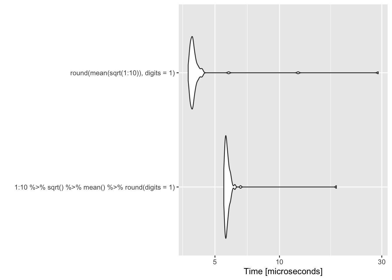

You must stay hyper-alert as to the names in the data frame you are working with. You might not have created this data frame. This may be a function you wrote to take any data frame from a user…. Otherwise, bad things like this can happen.

fun <- function(x, cyl=1){
x %>% transform(new = mpg^cyl) %>% select(mpg, new)
}

Works great!

df <- data.frame(mpg=runif(10, 10, 30))
fun(df, cyl=0.5)

##         mpg      new
## 1  15.15951 3.893521
## 2  26.76402 5.173396
## 3  17.31408 4.161019
## 4  17.62835 4.198613
## 5  26.68647 5.165895
## 6  13.99436 3.740903
## 7  13.71048 3.702767
## 8  15.80307 3.975307
## 9  17.29457 4.158674
## 10 15.84034 3.979992

Why, why? It didn’t complain but this is wrong!

fun(mtcars[1:5,], cyl=0.5)

##                    mpg          new
## Mazda RX4         21.0 8.576612e+07
## Mazda RX4 Wag     21.0 8.576612e+07
## Datsun 710        22.8 2.702336e+05
## Hornet 4 Drive    21.4 9.604674e+07
## Hornet Sportabout 18.7 1.495316e+10

Tidyverse verbs

Read up on tidyverse verbs here.

NOTE:

I am using piping because that is how you will see these verbs used in online material. They are just functions and you do not need to use them with piping.
They are very slow. For loops are not the place for these functions. apply() in base R is much faster.
Tidyverse is maturing and the semantics across functions is not quite the same. Careful.

Workflow

data.frame %>%
  select columns or filter rows %>%
  summarize or mutate

data.frame %>%
  group data %>%
  summarize or mutate

Verbs that we will learn:

select() select columns
filter() select rows
group_by() apply the function differently within groups.
summarize() apply function over columns -> fewer rows. Like apply(df,2,function)
mutate() apply function to columns and make new column. Like apply(df,1,function)

What we won’t learn: applying a function across a group of columns. See ?across to learn about that.

Selecting and filtering

data.frame %>%
  select or filter

`select()`

Select columns.

head(mtcars)

##                    mpg cyl disp  hp drat    wt  qsec vs am gear carb
## Mazda RX4         21.0   6  160 110 3.90 2.620 16.46  0  1    4    4
## Mazda RX4 Wag     21.0   6  160 110 3.90 2.875 17.02  0  1    4    4
## Datsun 710        22.8   4  108  93 3.85 2.320 18.61  1  1    4    1
## Hornet 4 Drive    21.4   6  258 110 3.08 3.215 19.44  1  0    3    1
## Hornet Sportabout 18.7   8  360 175 3.15 3.440 17.02  0  0    3    2
## Valiant           18.1   6  225 105 2.76 3.460 20.22  1  0    3    1

mtcars %>% select(mpg)

##                      mpg
## Mazda RX4           21.0
## Mazda RX4 Wag       21.0
## Datsun 710          22.8
## Hornet 4 Drive      21.4
## Hornet Sportabout   18.7
## Valiant             18.1
## Duster 360          14.3
## Merc 240D           24.4
## Merc 230            22.8
## Merc 280            19.2
## Merc 280C           17.8
## Merc 450SE          16.4
## Merc 450SL          17.3
## Merc 450SLC         15.2
## Cadillac Fleetwood  10.4
## Lincoln Continental 10.4
## Chrysler Imperial   14.7
## Fiat 128            32.4
## Honda Civic         30.4
## Toyota Corolla      33.9
## Toyota Corona       21.5
## Dodge Challenger    15.5
## AMC Javelin         15.2
## Camaro Z28          13.3
## Pontiac Firebird    19.2
## Fiat X1-9           27.3
## Porsche 914-2       26.0
## Lotus Europa        30.4
## Ford Pantera L      15.8
## Ferrari Dino        19.7
## Maserati Bora       15.0
## Volvo 142E          21.4

mtcars %>% select(-mpg, -qsec, -gear, -cyl)

##                      disp  hp drat    wt vs am carb
## Mazda RX4           160.0 110 3.90 2.620  0  1    4
## Mazda RX4 Wag       160.0 110 3.90 2.875  0  1    4
## Datsun 710          108.0  93 3.85 2.320  1  1    1
## Hornet 4 Drive      258.0 110 3.08 3.215  1  0    1
## Hornet Sportabout   360.0 175 3.15 3.440  0  0    2
## Valiant             225.0 105 2.76 3.460  1  0    1
## Duster 360          360.0 245 3.21 3.570  0  0    4
## Merc 240D           146.7  62 3.69 3.190  1  0    2
## Merc 230            140.8  95 3.92 3.150  1  0    2
## Merc 280            167.6 123 3.92 3.440  1  0    4
## Merc 280C           167.6 123 3.92 3.440  1  0    4
## Merc 450SE          275.8 180 3.07 4.070  0  0    3
## Merc 450SL          275.8 180 3.07 3.730  0  0    3
## Merc 450SLC         275.8 180 3.07 3.780  0  0    3
## Cadillac Fleetwood  472.0 205 2.93 5.250  0  0    4
## Lincoln Continental 460.0 215 3.00 5.424  0  0    4
## Chrysler Imperial   440.0 230 3.23 5.345  0  0    4
## Fiat 128             78.7  66 4.08 2.200  1  1    1
## Honda Civic          75.7  52 4.93 1.615  1  1    2
## Toyota Corolla       71.1  65 4.22 1.835  1  1    1
## Toyota Corona       120.1  97 3.70 2.465  1  0    1
## Dodge Challenger    318.0 150 2.76 3.520  0  0    2
## AMC Javelin         304.0 150 3.15 3.435  0  0    2
## Camaro Z28          350.0 245 3.73 3.840  0  0    4
## Pontiac Firebird    400.0 175 3.08 3.845  0  0    2
## Fiat X1-9            79.0  66 4.08 1.935  1  1    1
## Porsche 914-2       120.3  91 4.43 2.140  0  1    2
## Lotus Europa         95.1 113 3.77 1.513  1  1    2
## Ford Pantera L      351.0 264 4.22 3.170  0  1    4
## Ferrari Dino        145.0 175 3.62 2.770  0  1    6
## Maserati Bora       301.0 335 3.54 3.570  0  1    8
## Volvo 142E          121.0 109 4.11 2.780  1  1    2

mtcars %>% select(disp:qsec)

##                      disp  hp drat    wt  qsec
## Mazda RX4           160.0 110 3.90 2.620 16.46
## Mazda RX4 Wag       160.0 110 3.90 2.875 17.02
## Datsun 710          108.0  93 3.85 2.320 18.61
## Hornet 4 Drive      258.0 110 3.08 3.215 19.44
## Hornet Sportabout   360.0 175 3.15 3.440 17.02
## Valiant             225.0 105 2.76 3.460 20.22
## Duster 360          360.0 245 3.21 3.570 15.84
## Merc 240D           146.7  62 3.69 3.190 20.00
## Merc 230            140.8  95 3.92 3.150 22.90
## Merc 280            167.6 123 3.92 3.440 18.30
## Merc 280C           167.6 123 3.92 3.440 18.90
## Merc 450SE          275.8 180 3.07 4.070 17.40
## Merc 450SL          275.8 180 3.07 3.730 17.60
## Merc 450SLC         275.8 180 3.07 3.780 18.00
## Cadillac Fleetwood  472.0 205 2.93 5.250 17.98
## Lincoln Continental 460.0 215 3.00 5.424 17.82
## Chrysler Imperial   440.0 230 3.23 5.345 17.42
## Fiat 128             78.7  66 4.08 2.200 19.47
## Honda Civic          75.7  52 4.93 1.615 18.52
## Toyota Corolla       71.1  65 4.22 1.835 19.90
## Toyota Corona       120.1  97 3.70 2.465 20.01
## Dodge Challenger    318.0 150 2.76 3.520 16.87
## AMC Javelin         304.0 150 3.15 3.435 17.30
## Camaro Z28          350.0 245 3.73 3.840 15.41
## Pontiac Firebird    400.0 175 3.08 3.845 17.05
## Fiat X1-9            79.0  66 4.08 1.935 18.90
## Porsche 914-2       120.3  91 4.43 2.140 16.70
## Lotus Europa         95.1 113 3.77 1.513 16.90
## Ford Pantera L      351.0 264 4.22 3.170 14.50
## Ferrari Dino        145.0 175 3.62 2.770 15.50
## Maserati Bora       301.0 335 3.54 3.570 14.60
## Volvo 142E          121.0 109 4.11 2.780 18.60

mtcars %>% select(!disp:qsec)

##                      mpg cyl vs am gear carb
## Mazda RX4           21.0   6  0  1    4    4
## Mazda RX4 Wag       21.0   6  0  1    4    4
## Datsun 710          22.8   4  1  1    4    1
## Hornet 4 Drive      21.4   6  1  0    3    1
## Hornet Sportabout   18.7   8  0  0    3    2
## Valiant             18.1   6  1  0    3    1
## Duster 360          14.3   8  0  0    3    4
## Merc 240D           24.4   4  1  0    4    2
## Merc 230            22.8   4  1  0    4    2
## Merc 280            19.2   6  1  0    4    4
## Merc 280C           17.8   6  1  0    4    4
## Merc 450SE          16.4   8  0  0    3    3
## Merc 450SL          17.3   8  0  0    3    3
## Merc 450SLC         15.2   8  0  0    3    3
## Cadillac Fleetwood  10.4   8  0  0    3    4
## Lincoln Continental 10.4   8  0  0    3    4
## Chrysler Imperial   14.7   8  0  0    3    4
## Fiat 128            32.4   4  1  1    4    1
## Honda Civic         30.4   4  1  1    4    2
## Toyota Corolla      33.9   4  1  1    4    1
## Toyota Corona       21.5   4  1  0    3    1
## Dodge Challenger    15.5   8  0  0    3    2
## AMC Javelin         15.2   8  0  0    3    2
## Camaro Z28          13.3   8  0  0    3    4
## Pontiac Firebird    19.2   8  0  0    3    2
## Fiat X1-9           27.3   4  1  1    4    1
## Porsche 914-2       26.0   4  0  1    5    2
## Lotus Europa        30.4   4  1  1    5    2
## Ford Pantera L      15.8   8  0  1    5    4
## Ferrari Dino        19.7   6  0  1    5    6
## Maserati Bora       15.0   8  0  1    5    8
## Volvo 142E          21.4   4  1  1    4    2

df %>% select(where(is.numeric))

##         mpg
## 1  15.15951
## 2  26.76402
## 3  17.31408
## 4  17.62835
## 5  26.68647
## 6  13.99436
## 7  13.71048
## 8  15.80307
## 9  17.29457
## 10 15.84034

`filter()`

Select rows.

mtcars %>% filter(cyl==4)

##                 mpg cyl  disp  hp drat    wt  qsec vs am gear carb
## Datsun 710     22.8   4 108.0  93 3.85 2.320 18.61  1  1    4    1
## Merc 240D      24.4   4 146.7  62 3.69 3.190 20.00  1  0    4    2
## Merc 230       22.8   4 140.8  95 3.92 3.150 22.90  1  0    4    2
## Fiat 128       32.4   4  78.7  66 4.08 2.200 19.47  1  1    4    1
## Honda Civic    30.4   4  75.7  52 4.93 1.615 18.52  1  1    4    2
## Toyota Corolla 33.9   4  71.1  65 4.22 1.835 19.90  1  1    4    1
## Toyota Corona  21.5   4 120.1  97 3.70 2.465 20.01  1  0    3    1
## Fiat X1-9      27.3   4  79.0  66 4.08 1.935 18.90  1  1    4    1
## Porsche 914-2  26.0   4 120.3  91 4.43 2.140 16.70  0  1    5    2
## Lotus Europa   30.4   4  95.1 113 3.77 1.513 16.90  1  1    5    2
## Volvo 142E     21.4   4 121.0 109 4.11 2.780 18.60  1  1    4    2

Same as subset(df, cyl==4) or df[df$cyl==4,]

mtcars %>% filter(cyl==4, hp>90)

##                mpg cyl  disp  hp drat    wt  qsec vs am gear carb
## Datsun 710    22.8   4 108.0  93 3.85 2.320 18.61  1  1    4    1
## Merc 230      22.8   4 140.8  95 3.92 3.150 22.90  1  0    4    2
## Toyota Corona 21.5   4 120.1  97 3.70 2.465 20.01  1  0    3    1
## Porsche 914-2 26.0   4 120.3  91 4.43 2.140 16.70  0  1    5    2
## Lotus Europa  30.4   4  95.1 113 3.77 1.513 16.90  1  1    5    2
## Volvo 142E    21.4   4 121.0 109 4.11 2.780 18.60  1  1    4    2

Same as subset(df, cyl==4 & hp>90) or df[df$cyl==4 & df$hp>90,].

`summarize()`

summarize() summarizes down columns and leads to fewer rows. You must tell it the columns to work on.

data.frame %>%
  summarize

Apply a function to columns.

mtcars %>% 
  summarize(mean.wt=mean(wt))

##   mean.wt
## 1 3.21725

I can add on more functions.

mtcars %>% 
  summarize(mean.wt=mean(wt)) %>%
  round(digits=2)

##   mean.wt
## 1    3.22

Same as

round(mean(mtcars$wt), digits=2)

## [1] 3.22

You can specify multiple columns. You have to put in c() in this case.

mtcars %>% 
  summarize(mean.wt=mean(c(mpg, hp)))

##    mean.wt
## 1 83.38906

Same as

mean(c(mtcars$mpg, mtcars$hp))

## [1] 83.38906

Sadly this does NOT work for specifying a range. It computes something but not what you’d think. This is the apply across columns case. Read up on that in ?across.

mtcars %>% 
  summarize(mean.wt=mean(mpg:hp))

## Warning in mpg:hp: numerical expression has 32 elements: only the first used

## Warning in mpg:hp: numerical expression has 32 elements: only the first used

##   mean.wt
## 1    65.5

This is computing the mean of this:

mtcars[1,"mpg"]:mtcars[1,"hp"]

##  [1]  21  22  23  24  25  26  27  28  29  30  31  32  33  34  35  36  37  38  39
## [20]  40  41  42  43  44  45  46  47  48  49  50  51  52  53  54  55  56  57  58
## [39]  59  60  61  62  63  64  65  66  67  68  69  70  71  72  73  74  75  76  77
## [58]  78  79  80  81  82  83  84  85  86  87  88  89  90  91  92  93  94  95  96
## [77]  97  98  99 100 101 102 103 104 105 106 107 108 109 110

which is

mean(mtcars[1,"mpg"]:mtcars[1,"hp"])

## [1] 65.5

`summarize()` by column

summarize_all() and summarize_at()

Apply to a range of columns or all columns. Note the _at() and _all() functions have been superseded with across() but I find across() really cumbersome. I personally would use select() and summarize_all().

mtcars %>% summarize_at(vars(mpg:hp), mean)

##        mpg    cyl     disp       hp
## 1 20.09062 6.1875 230.7219 146.6875

data.frame %>%
  select columns %>%
  use summarize_all()

mtcars %>% 
  select(mpg:hp) %>% 
  summarize_all(mean)

##        mpg    cyl     disp       hp
## 1 20.09062 6.1875 230.7219 146.6875

apply(mtcars[,1:4],2,mean)

##       mpg       cyl      disp        hp 
##  20.09062   6.18750 230.72188 146.68750

summarize_all() is less picky than apply()

df <- mtcars[,1:3]; df$label="test"
df %>% summarize_all(mean)

## Warning in mean.default(label): argument is not numeric or logical: returning NA

##        mpg    cyl     disp label
## 1 20.09062 6.1875 230.7219    NA

while apply() gives all NA.

apply(df,2,mean)

## Warning in mean.default(newX[, i], ...): argument is not numeric or logical:
## returning NA

## Warning in mean.default(newX[, i], ...): argument is not numeric or logical:
## returning NA

## Warning in mean.default(newX[, i], ...): argument is not numeric or logical:
## returning NA

## Warning in mean.default(newX[, i], ...): argument is not numeric or logical:
## returning NA

##   mpg   cyl  disp label 
##    NA    NA    NA    NA

Another example.

data.frame %>%
  select rows %>%
  select columns %>%
  use summarize_all() verb to apply %>%
  format with round()

mtcars %>% 
  filter(cyl==4) %>% 
  select(mpg:hp) %>% 
  summarize_all(mean) %>%
  round(digits=2) %>%
  paste(collapse=" -- ")

## [1] "26.66 -- 4 -- 105.14 -- 82.64"

`summarize()` by group

data.frame %>%
  define groups %>%
  apply summarize within groups

df2 <- data.frame(id=paste0(rep("s",8),1:2),
                  pop=paste0(rep("r",8),rep(1:2,each=4)),
                  Week1=rnorm(8), Week2=rnorm(8), Week3=rnorm(8), Week4=rnorm(8))
head(df2)

##   id pop       Week1       Week2      Week3      Week4
## 1 s1  r1 -0.83551483  1.43965277  1.6664183 -1.1372446
## 2 s2  r1 -1.63488346  0.94898124 -0.6758438  0.4264061
## 3 s1  r1 -0.04529889  0.57412587 -1.1827151 -0.2683061
## 4 s2  r1 -0.19604077  0.01420002  1.2047887 -0.8967390
## 5 s1  r2 -0.71715376 -1.28082258 -0.8366131 -0.1310937
## 6 s2  r2 -0.78223915 -1.39280749  1.1294121 -1.2896710

The group_by() function allows you to do more complicated things. Take the mean by pop.

df2 %>% group_by(pop) %>% summarize_all(mean)

## Warning in mean.default(id): argument is not numeric or logical: returning NA

## Warning in mean.default(id): argument is not numeric or logical: returning NA

## # A tibble: 2 x 6
##   pop      id   Week1  Week2 Week3  Week4
## * <chr> <dbl>   <dbl>  <dbl> <dbl>  <dbl>
## 1 r1       NA -0.678   0.744 0.253 -0.469
## 2 r2       NA  0.0901 -0.682 0.607 -0.676

apply(df2[df2$pop=="r1",3:6],2,mean)

##      Week1      Week2      Week3      Week4 
## -0.6779345  0.7442400  0.2531620 -0.4689709

Take the mean for all weeks by pop and id. Notice that I have to specify columns for summarize().

df2 %>% 
  group_by(pop, id) %>%
  summarize(mean=mean(c(Week1, Week2, Week3, Week4)))

## `summarise()` has grouped output by 'pop'. You can override using the `.groups` argument.

## # A tibble: 4 x 3
## # Groups:   pop [2]
##   pop   id       mean
##   <chr> <chr>   <dbl>
## 1 r1    s1     0.0264
## 2 r1    s2    -0.101 
## 3 r2    s1    -0.480 
## 4 r2    s2     0.149

Combine group and select

Select based on properties. For some reason you have to wrap in where().

df2 %>% group_by(pop) %>% 
  select(where(is.numeric)) %>% 
  summarize_all(mean)

## Adding missing grouping variables: `pop`

## # A tibble: 2 x 5
##   pop     Week1  Week2 Week3  Week4
## * <chr>   <dbl>  <dbl> <dbl>  <dbl>
## 1 r1    -0.678   0.744 0.253 -0.469
## 2 r2     0.0901 -0.682 0.607 -0.676

Select based on name.

df2 %>% group_by(pop) %>% 
  select(ends_with("2")) %>% 
  summarize_all(mean)

## Adding missing grouping variables: `pop`

## # A tibble: 2 x 2
##   pop    Week2
## * <chr>  <dbl>
## 1 r1     0.744
## 2 r2    -0.682

`mutate()`

Apply a function across rows and return a new column. Like apply(df,1,fun).

mtcars %>% 
   select(mpg:wt) %>%
   mutate(wt.hp=wt/hp)

##                      mpg cyl  disp  hp drat    wt      wt.hp
## Mazda RX4           21.0   6 160.0 110 3.90 2.620 0.02381818
## Mazda RX4 Wag       21.0   6 160.0 110 3.90 2.875 0.02613636
## Datsun 710          22.8   4 108.0  93 3.85 2.320 0.02494624
## Hornet 4 Drive      21.4   6 258.0 110 3.08 3.215 0.02922727
## Hornet Sportabout   18.7   8 360.0 175 3.15 3.440 0.01965714
## Valiant             18.1   6 225.0 105 2.76 3.460 0.03295238
## Duster 360          14.3   8 360.0 245 3.21 3.570 0.01457143
## Merc 240D           24.4   4 146.7  62 3.69 3.190 0.05145161
## Merc 230            22.8   4 140.8  95 3.92 3.150 0.03315789
## Merc 280            19.2   6 167.6 123 3.92 3.440 0.02796748
## Merc 280C           17.8   6 167.6 123 3.92 3.440 0.02796748
## Merc 450SE          16.4   8 275.8 180 3.07 4.070 0.02261111
## Merc 450SL          17.3   8 275.8 180 3.07 3.730 0.02072222
## Merc 450SLC         15.2   8 275.8 180 3.07 3.780 0.02100000
## Cadillac Fleetwood  10.4   8 472.0 205 2.93 5.250 0.02560976
## Lincoln Continental 10.4   8 460.0 215 3.00 5.424 0.02522791
## Chrysler Imperial   14.7   8 440.0 230 3.23 5.345 0.02323913
## Fiat 128            32.4   4  78.7  66 4.08 2.200 0.03333333
## Honda Civic         30.4   4  75.7  52 4.93 1.615 0.03105769
## Toyota Corolla      33.9   4  71.1  65 4.22 1.835 0.02823077
## Toyota Corona       21.5   4 120.1  97 3.70 2.465 0.02541237
## Dodge Challenger    15.5   8 318.0 150 2.76 3.520 0.02346667
## AMC Javelin         15.2   8 304.0 150 3.15 3.435 0.02290000
## Camaro Z28          13.3   8 350.0 245 3.73 3.840 0.01567347
## Pontiac Firebird    19.2   8 400.0 175 3.08 3.845 0.02197143
## Fiat X1-9           27.3   4  79.0  66 4.08 1.935 0.02931818
## Porsche 914-2       26.0   4 120.3  91 4.43 2.140 0.02351648
## Lotus Europa        30.4   4  95.1 113 3.77 1.513 0.01338938
## Ford Pantera L      15.8   8 351.0 264 4.22 3.170 0.01200758
## Ferrari Dino        19.7   6 145.0 175 3.62 2.770 0.01582857
## Maserati Bora       15.0   8 301.0 335 3.54 3.570 0.01065672
## Volvo 142E          21.4   4 121.0 109 4.11 2.780 0.02550459

You can write custom functions to apply to the groups.

fun <- function(x,y){fit <- lm(y~x); coef(fit)[1]} #return interept
mtcars %>% 
  group_by(carb) %>% 
  summarize(lmm=fun(mpg,hp))

## # A tibble: 6 x 2
##    carb   lmm
## * <dbl> <dbl>
## 1     1  162.
## 2     2  252.
## 3     3  180.
## 4     4  379.
## 5     6  175 
## 6     8  335

Use mutate() to add column. This will not change the number of rows.

mtcars %>% 
  group_by(carb) %>% 
  mutate(lmm=fun(mpg,hp)) %>%
  select(mpg, hp, lmm)

## Adding missing grouping variables: `carb`

## # A tibble: 32 x 4
## # Groups:   carb [6]
##     carb   mpg    hp   lmm
##    <dbl> <dbl> <dbl> <dbl>
##  1     4  21     110  379.
##  2     4  21     110  379.
##  3     1  22.8    93  162.
##  4     1  21.4   110  162.
##  5     2  18.7   175  252.
##  6     1  18.1   105  162.
##  7     4  14.3   245  379.
##  8     2  24.4    62  252.
##  9     2  22.8    95  252.
## 10     4  19.2   123  379.
## # … with 22 more rows

Careful `mutate()` guesses

That works.

mtcars %>% 
   select(mpg:wt) %>%
   mutate(mean=sqrt(wt))

##                      mpg cyl  disp  hp drat    wt     mean
## Mazda RX4           21.0   6 160.0 110 3.90 2.620 1.618641
## Mazda RX4 Wag       21.0   6 160.0 110 3.90 2.875 1.695582
## Datsun 710          22.8   4 108.0  93 3.85 2.320 1.523155
## Hornet 4 Drive      21.4   6 258.0 110 3.08 3.215 1.793042
## Hornet Sportabout   18.7   8 360.0 175 3.15 3.440 1.854724
## Valiant             18.1   6 225.0 105 2.76 3.460 1.860108
## Duster 360          14.3   8 360.0 245 3.21 3.570 1.889444
## Merc 240D           24.4   4 146.7  62 3.69 3.190 1.786057
## Merc 230            22.8   4 140.8  95 3.92 3.150 1.774824
## Merc 280            19.2   6 167.6 123 3.92 3.440 1.854724
## Merc 280C           17.8   6 167.6 123 3.92 3.440 1.854724
## Merc 450SE          16.4   8 275.8 180 3.07 4.070 2.017424
## Merc 450SL          17.3   8 275.8 180 3.07 3.730 1.931321
## Merc 450SLC         15.2   8 275.8 180 3.07 3.780 1.944222
## Cadillac Fleetwood  10.4   8 472.0 205 2.93 5.250 2.291288
## Lincoln Continental 10.4   8 460.0 215 3.00 5.424 2.328948
## Chrysler Imperial   14.7   8 440.0 230 3.23 5.345 2.311926
## Fiat 128            32.4   4  78.7  66 4.08 2.200 1.483240
## Honda Civic         30.4   4  75.7  52 4.93 1.615 1.270827
## Toyota Corolla      33.9   4  71.1  65 4.22 1.835 1.354622
## Toyota Corona       21.5   4 120.1  97 3.70 2.465 1.570032
## Dodge Challenger    15.5   8 318.0 150 2.76 3.520 1.876166
## AMC Javelin         15.2   8 304.0 150 3.15 3.435 1.853375
## Camaro Z28          13.3   8 350.0 245 3.73 3.840 1.959592
## Pontiac Firebird    19.2   8 400.0 175 3.08 3.845 1.960867
## Fiat X1-9           27.3   4  79.0  66 4.08 1.935 1.391043
## Porsche 914-2       26.0   4 120.3  91 4.43 2.140 1.462874
## Lotus Europa        30.4   4  95.1 113 3.77 1.513 1.230041
## Ford Pantera L      15.8   8 351.0 264 4.22 3.170 1.780449
## Ferrari Dino        19.7   6 145.0 175 3.62 2.770 1.664332
## Maserati Bora       15.0   8 301.0 335 3.54 3.570 1.889444
## Volvo 142E          21.4   4 121.0 109 4.11 2.780 1.667333

Yipes! It decided you must want me to take the mean in the whole column.

mtcars %>% 
   select(mpg:wt) %>%
   mutate(mean=mean(wt))

##                      mpg cyl  disp  hp drat    wt    mean
## Mazda RX4           21.0   6 160.0 110 3.90 2.620 3.21725
## Mazda RX4 Wag       21.0   6 160.0 110 3.90 2.875 3.21725
## Datsun 710          22.8   4 108.0  93 3.85 2.320 3.21725
## Hornet 4 Drive      21.4   6 258.0 110 3.08 3.215 3.21725
## Hornet Sportabout   18.7   8 360.0 175 3.15 3.440 3.21725
## Valiant             18.1   6 225.0 105 2.76 3.460 3.21725
## Duster 360          14.3   8 360.0 245 3.21 3.570 3.21725
## Merc 240D           24.4   4 146.7  62 3.69 3.190 3.21725
## Merc 230            22.8   4 140.8  95 3.92 3.150 3.21725
## Merc 280            19.2   6 167.6 123 3.92 3.440 3.21725
## Merc 280C           17.8   6 167.6 123 3.92 3.440 3.21725
## Merc 450SE          16.4   8 275.8 180 3.07 4.070 3.21725
## Merc 450SL          17.3   8 275.8 180 3.07 3.730 3.21725
## Merc 450SLC         15.2   8 275.8 180 3.07 3.780 3.21725
## Cadillac Fleetwood  10.4   8 472.0 205 2.93 5.250 3.21725
## Lincoln Continental 10.4   8 460.0 215 3.00 5.424 3.21725
## Chrysler Imperial   14.7   8 440.0 230 3.23 5.345 3.21725
## Fiat 128            32.4   4  78.7  66 4.08 2.200 3.21725
## Honda Civic         30.4   4  75.7  52 4.93 1.615 3.21725
## Toyota Corolla      33.9   4  71.1  65 4.22 1.835 3.21725
## Toyota Corona       21.5   4 120.1  97 3.70 2.465 3.21725
## Dodge Challenger    15.5   8 318.0 150 2.76 3.520 3.21725
## AMC Javelin         15.2   8 304.0 150 3.15 3.435 3.21725
## Camaro Z28          13.3   8 350.0 245 3.73 3.840 3.21725
## Pontiac Firebird    19.2   8 400.0 175 3.08 3.845 3.21725
## Fiat X1-9           27.3   4  79.0  66 4.08 1.935 3.21725
## Porsche 914-2       26.0   4 120.3  91 4.43 2.140 3.21725
## Lotus Europa        30.4   4  95.1 113 3.77 1.513 3.21725
## Ford Pantera L      15.8   8 351.0 264 4.22 3.170 3.21725
## Ferrari Dino        19.7   6 145.0 175 3.62 2.770 3.21725
## Maserati Bora       15.0   8 301.0 335 3.54 3.570 3.21725
## Volvo 142E          21.4   4 121.0 109 4.11 2.780 3.21725

Careful regarding across

It is super easy to try to use this to apply functions across multiple columns. Doesn’t work. You need to use ?across (or group_by() with a row factor).

mtcars %>% 
   select(mpg:wt) %>%
   mutate(mean1 = (wt+hp)/2, mean2=mean(c(wt,hp)))

##                      mpg cyl  disp  hp drat    wt    mean1    mean2
## Mazda RX4           21.0   6 160.0 110 3.90 2.620  56.3100 74.95238
## Mazda RX4 Wag       21.0   6 160.0 110 3.90 2.875  56.4375 74.95238
## Datsun 710          22.8   4 108.0  93 3.85 2.320  47.6600 74.95238
## Hornet 4 Drive      21.4   6 258.0 110 3.08 3.215  56.6075 74.95238
## Hornet Sportabout   18.7   8 360.0 175 3.15 3.440  89.2200 74.95238
## Valiant             18.1   6 225.0 105 2.76 3.460  54.2300 74.95238
## Duster 360          14.3   8 360.0 245 3.21 3.570 124.2850 74.95238
## Merc 240D           24.4   4 146.7  62 3.69 3.190  32.5950 74.95238
## Merc 230            22.8   4 140.8  95 3.92 3.150  49.0750 74.95238
## Merc 280            19.2   6 167.6 123 3.92 3.440  63.2200 74.95238
## Merc 280C           17.8   6 167.6 123 3.92 3.440  63.2200 74.95238
## Merc 450SE          16.4   8 275.8 180 3.07 4.070  92.0350 74.95238
## Merc 450SL          17.3   8 275.8 180 3.07 3.730  91.8650 74.95238
## Merc 450SLC         15.2   8 275.8 180 3.07 3.780  91.8900 74.95238
## Cadillac Fleetwood  10.4   8 472.0 205 2.93 5.250 105.1250 74.95238
## Lincoln Continental 10.4   8 460.0 215 3.00 5.424 110.2120 74.95238
## Chrysler Imperial   14.7   8 440.0 230 3.23 5.345 117.6725 74.95238
## Fiat 128            32.4   4  78.7  66 4.08 2.200  34.1000 74.95238
## Honda Civic         30.4   4  75.7  52 4.93 1.615  26.8075 74.95238
## Toyota Corolla      33.9   4  71.1  65 4.22 1.835  33.4175 74.95238
## Toyota Corona       21.5   4 120.1  97 3.70 2.465  49.7325 74.95238
## Dodge Challenger    15.5   8 318.0 150 2.76 3.520  76.7600 74.95238
## AMC Javelin         15.2   8 304.0 150 3.15 3.435  76.7175 74.95238
## Camaro Z28          13.3   8 350.0 245 3.73 3.840 124.4200 74.95238
## Pontiac Firebird    19.2   8 400.0 175 3.08 3.845  89.4225 74.95238
## Fiat X1-9           27.3   4  79.0  66 4.08 1.935  33.9675 74.95238
## Porsche 914-2       26.0   4 120.3  91 4.43 2.140  46.5700 74.95238
## Lotus Europa        30.4   4  95.1 113 3.77 1.513  57.2565 74.95238
## Ford Pantera L      15.8   8 351.0 264 4.22 3.170 133.5850 74.95238
## Ferrari Dino        19.7   6 145.0 175 3.62 2.770  88.8850 74.95238
## Maserati Bora       15.0   8 301.0 335 3.54 3.570 169.2850 74.95238
## Volvo 142E          21.4   4 121.0 109 4.11 2.780  55.8900 74.95238

Tidyverse verbs are slow

For loops are not the place for these verbs!

bm <- microbenchmark(
  apply(mtcars,2,sum), 
  summarize_all(mtcars, sum)
  )
ggplot2::autoplot(bm)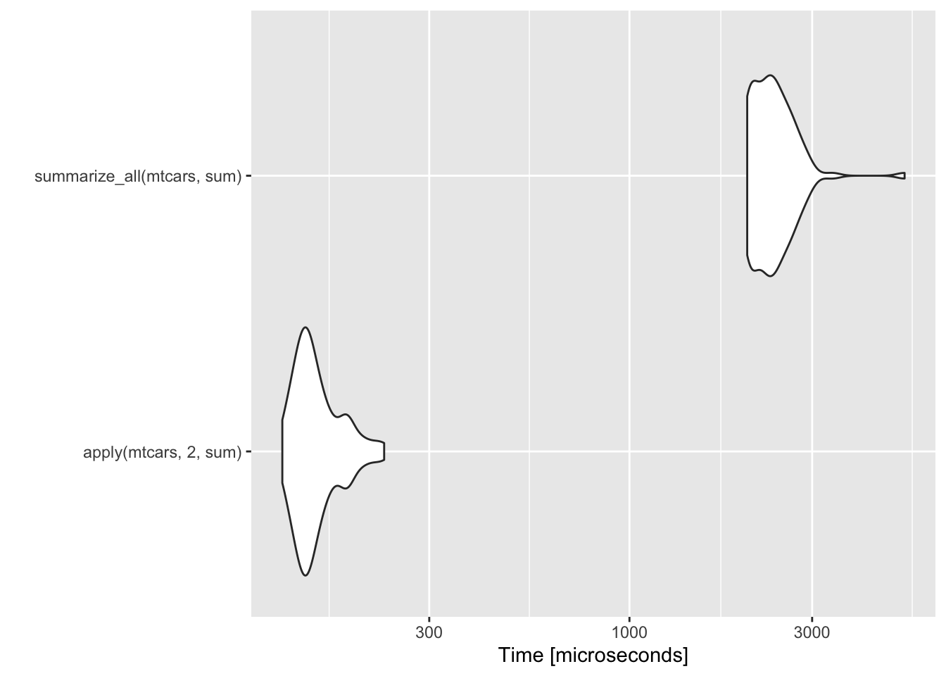

bm <- microbenchmark(
   mtcars[mtcars$cyl==4,], 
   filter(mtcars, cyl==4),
    subset(mtcars, cyl==4)
   )
ggplot2::autoplot(bm)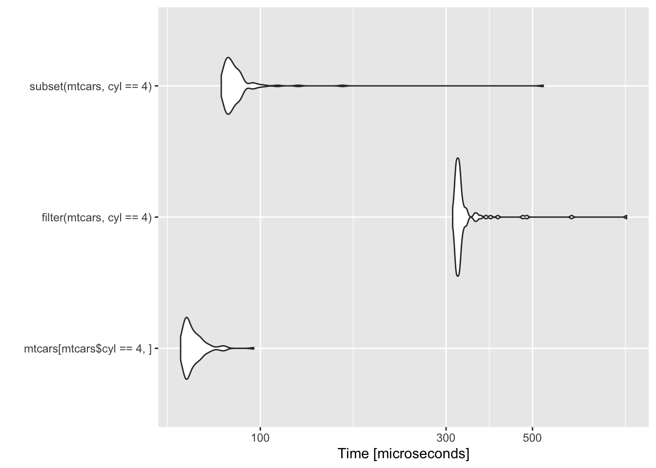

Long and wide data frames

Wide is what you need for say lm(). You have your response variable in one column and then your predictor variables in other columns.

df <- subset(mtcars, select=c(mpg, wt, hp, carb))
df$model <- rownames(mtcars)
head(df)

##                    mpg    wt  hp carb             model
## Mazda RX4         21.0 2.620 110    4         Mazda RX4
## Mazda RX4 Wag     21.0 2.875 110    4     Mazda RX4 Wag
## Datsun 710        22.8 2.320  93    1        Datsun 710
## Hornet 4 Drive    21.4 3.215 110    1    Hornet 4 Drive
## Hornet Sportabout 18.7 3.440 175    2 Hornet Sportabout
## Valiant           18.1 3.460 105    1           Valiant

Fit with lm().

fit <- lm(mpg ~ wt + hp, data=df)
summary(fit)

## 
## Call:
## lm(formula = mpg ~ wt + hp, data = df)
## 
## Residuals:
##    Min     1Q Median     3Q    Max 
## -3.941 -1.600 -0.182  1.050  5.854 
## 
## Coefficients:
##             Estimate Std. Error t value Pr(>|t|)    
## (Intercept) 37.22727    1.59879  23.285  < 2e-16 ***
## wt          -3.87783    0.63273  -6.129 1.12e-06 ***
## hp          -0.03177    0.00903  -3.519  0.00145 ** 
## ---
## Signif. codes:  0 '***' 0.001 '**' 0.01 '*' 0.05 '.' 0.1 ' ' 1
## 
## Residual standard error: 2.593 on 29 degrees of freedom
## Multiple R-squared:  0.8268, Adjusted R-squared:  0.8148 
## F-statistic: 69.21 on 2 and 29 DF,  p-value: 9.109e-12

Long form is what ggplot wants. Usually I have to ponder a bit before I decide how to make my long form data frame. There is not just “one” that you could make from your wide form data frame.

Let’s make a plot of the red, green and blue columns. We want the points to be red, green or blue.

plot(df$mpg, col="red", ylim=c(0,200))
points(df$wt, col="green")
points(df$hp, col="blue")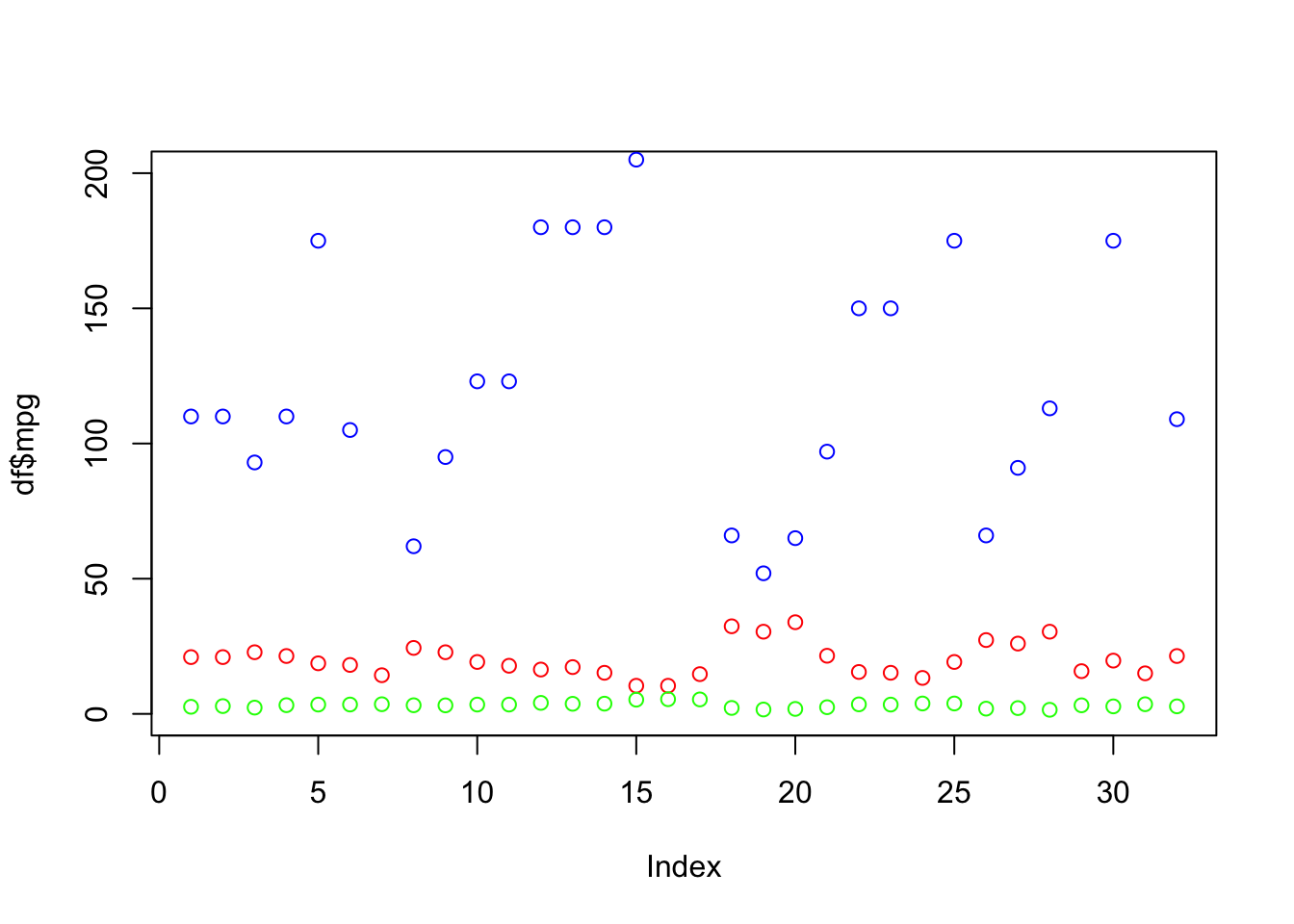

Same idea but let’s plot versus the carburator number. Let’s make a plot of the red, green and blue columns. We want the points to be red, green or blue.

plot(df$carb, df$mpg, col="red", ylim=c(0,200))
points(df$carb, df$wt, col="green")
points(df$carb, df$hp, col="blue")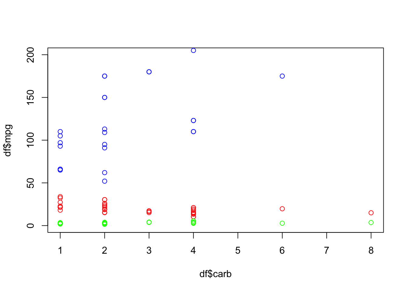

Now let’s do this in ggplot. What values do we want in the aes() function? Those need to be columns. aes(x=..., y=..., col=....)

data.frame(
   col=name.of.thing.we.plot, 
   y=value.of.thing.we.plot, 
   x=x.value
   )

So we’ll have a column of x (carb or model or 1:n), a column for our y (mpg,wt,hp) and a column for names (“mpg”,“wt”,“hb”).

df.long <- data.frame()
a <- data.frame(model=df$model, val=df$mpg, name="mpg", carb=df$carb)
df.long <- rbind(df.long, a)
a <- data.frame(model=df$model, val=df$wt, name="wt", carb=df$carb)
df.long <- rbind(df.long, a)
a <- data.frame(model=df$model, val=df$hp, name="hp", carb=df$carb)
df.long <- rbind(df.long, a)
df.long

##                  model     val name carb
## 1            Mazda RX4  21.000  mpg    4
## 2        Mazda RX4 Wag  21.000  mpg    4
## 3           Datsun 710  22.800  mpg    1
## 4       Hornet 4 Drive  21.400  mpg    1
## 5    Hornet Sportabout  18.700  mpg    2
## 6              Valiant  18.100  mpg    1
## 7           Duster 360  14.300  mpg    4
## 8            Merc 240D  24.400  mpg    2
## 9             Merc 230  22.800  mpg    2
## 10            Merc 280  19.200  mpg    4
## 11           Merc 280C  17.800  mpg    4
## 12          Merc 450SE  16.400  mpg    3
## 13          Merc 450SL  17.300  mpg    3
## 14         Merc 450SLC  15.200  mpg    3
## 15  Cadillac Fleetwood  10.400  mpg    4
## 16 Lincoln Continental  10.400  mpg    4
## 17   Chrysler Imperial  14.700  mpg    4
## 18            Fiat 128  32.400  mpg    1
## 19         Honda Civic  30.400  mpg    2
## 20      Toyota Corolla  33.900  mpg    1
## 21       Toyota Corona  21.500  mpg    1
## 22    Dodge Challenger  15.500  mpg    2
## 23         AMC Javelin  15.200  mpg    2
## 24          Camaro Z28  13.300  mpg    4
## 25    Pontiac Firebird  19.200  mpg    2
## 26           Fiat X1-9  27.300  mpg    1
## 27       Porsche 914-2  26.000  mpg    2
## 28        Lotus Europa  30.400  mpg    2
## 29      Ford Pantera L  15.800  mpg    4
## 30        Ferrari Dino  19.700  mpg    6
## 31       Maserati Bora  15.000  mpg    8
## 32          Volvo 142E  21.400  mpg    2
## 33           Mazda RX4   2.620   wt    4
## 34       Mazda RX4 Wag   2.875   wt    4
## 35          Datsun 710   2.320   wt    1
## 36      Hornet 4 Drive   3.215   wt    1
## 37   Hornet Sportabout   3.440   wt    2
## 38             Valiant   3.460   wt    1
## 39          Duster 360   3.570   wt    4
## 40           Merc 240D   3.190   wt    2
## 41            Merc 230   3.150   wt    2
## 42            Merc 280   3.440   wt    4
## 43           Merc 280C   3.440   wt    4
## 44          Merc 450SE   4.070   wt    3
## 45          Merc 450SL   3.730   wt    3
## 46         Merc 450SLC   3.780   wt    3
## 47  Cadillac Fleetwood   5.250   wt    4
## 48 Lincoln Continental   5.424   wt    4
## 49   Chrysler Imperial   5.345   wt    4
## 50            Fiat 128   2.200   wt    1
## 51         Honda Civic   1.615   wt    2
## 52      Toyota Corolla   1.835   wt    1
## 53       Toyota Corona   2.465   wt    1
## 54    Dodge Challenger   3.520   wt    2
## 55         AMC Javelin   3.435   wt    2
## 56          Camaro Z28   3.840   wt    4
## 57    Pontiac Firebird   3.845   wt    2
## 58           Fiat X1-9   1.935   wt    1
## 59       Porsche 914-2   2.140   wt    2
## 60        Lotus Europa   1.513   wt    2
## 61      Ford Pantera L   3.170   wt    4
## 62        Ferrari Dino   2.770   wt    6
## 63       Maserati Bora   3.570   wt    8
## 64          Volvo 142E   2.780   wt    2
## 65           Mazda RX4 110.000   hp    4
## 66       Mazda RX4 Wag 110.000   hp    4
## 67          Datsun 710  93.000   hp    1
## 68      Hornet 4 Drive 110.000   hp    1
## 69   Hornet Sportabout 175.000   hp    2
## 70             Valiant 105.000   hp    1
## 71          Duster 360 245.000   hp    4
## 72           Merc 240D  62.000   hp    2
## 73            Merc 230  95.000   hp    2
## 74            Merc 280 123.000   hp    4
## 75           Merc 280C 123.000   hp    4
## 76          Merc 450SE 180.000   hp    3
## 77          Merc 450SL 180.000   hp    3
## 78         Merc 450SLC 180.000   hp    3
## 79  Cadillac Fleetwood 205.000   hp    4
## 80 Lincoln Continental 215.000   hp    4
## 81   Chrysler Imperial 230.000   hp    4
## 82            Fiat 128  66.000   hp    1
## 83         Honda Civic  52.000   hp    2
## 84      Toyota Corolla  65.000   hp    1
## 85       Toyota Corona  97.000   hp    1
## 86    Dodge Challenger 150.000   hp    2
## 87         AMC Javelin 150.000   hp    2
## 88          Camaro Z28 245.000   hp    4
## 89    Pontiac Firebird 175.000   hp    2
## 90           Fiat X1-9  66.000   hp    1
## 91       Porsche 914-2  91.000   hp    2
## 92        Lotus Europa 113.000   hp    2
## 93      Ford Pantera L 264.000   hp    4
## 94        Ferrari Dino 175.000   hp    6
## 95       Maserati Bora 335.000   hp    8
## 96          Volvo 142E 109.000   hp    2

Now we can plot with ggplot.

ggplot(df.long, aes(x=model, y=val, col=name)) + geom_point()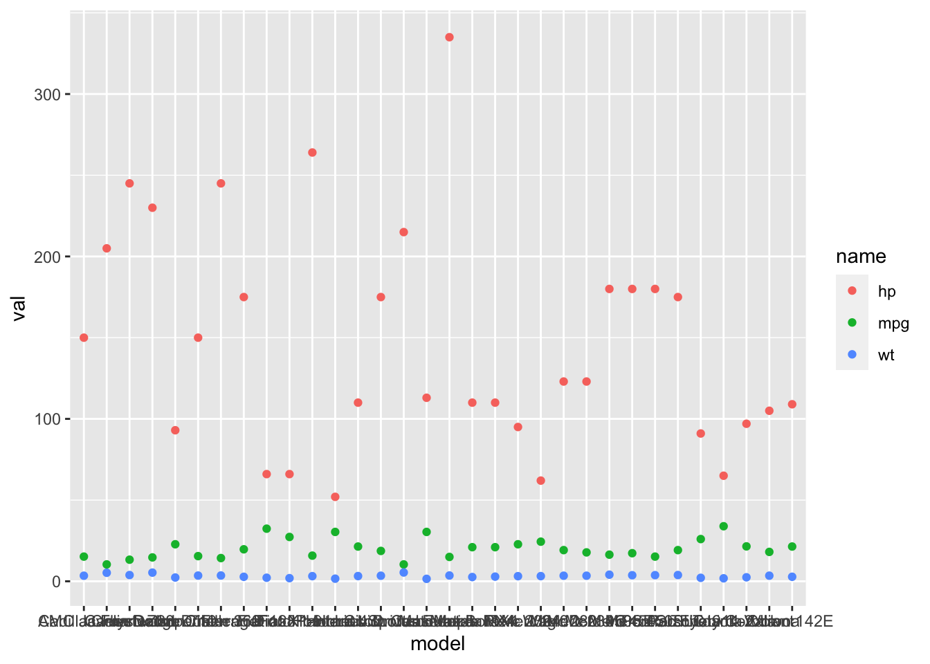

And we can easily do panels.

ggplot(df.long, aes(x=model, y=val, col=name)) + geom_point() +
  facet_wrap(~name)

Pivoting

So creating your long data frames like that would get tidieous and inefficient. The tidyr package has functions to make this easier.

`pivot_longer`

pivot_longer(
    data frame name,
    cols = what columns will you stack or pivot,
    names_to = colname for the column with the column names that your stacked,
    values_to = colname for the column with the values
  )

df.long2 <- 
  pivot_longer(
    df,
    cols = c("mpg", "wt", "hp"),
    names_to = "name",
    values_to = "val"
  )

df.long2

## # A tibble: 96 x 4
##     carb model          name     val
##    <dbl> <chr>          <chr>  <dbl>
##  1     4 Mazda RX4      mpg    21   
##  2     4 Mazda RX4      wt      2.62
##  3     4 Mazda RX4      hp    110   
##  4     4 Mazda RX4 Wag  mpg    21   
##  5     4 Mazda RX4 Wag  wt      2.88
##  6     4 Mazda RX4 Wag  hp    110   
##  7     1 Datsun 710     mpg    22.8 
##  8     1 Datsun 710     wt      2.32
##  9     1 Datsun 710     hp     93   
## 10     1 Hornet 4 Drive mpg    21.4 
## # … with 86 more rows

It changed the order our names but that’s ok. We can fix that if needed.

ggplot(df.long, aes(x=model, y=val, col=name)) + geom_point() +
  facet_wrap(~name)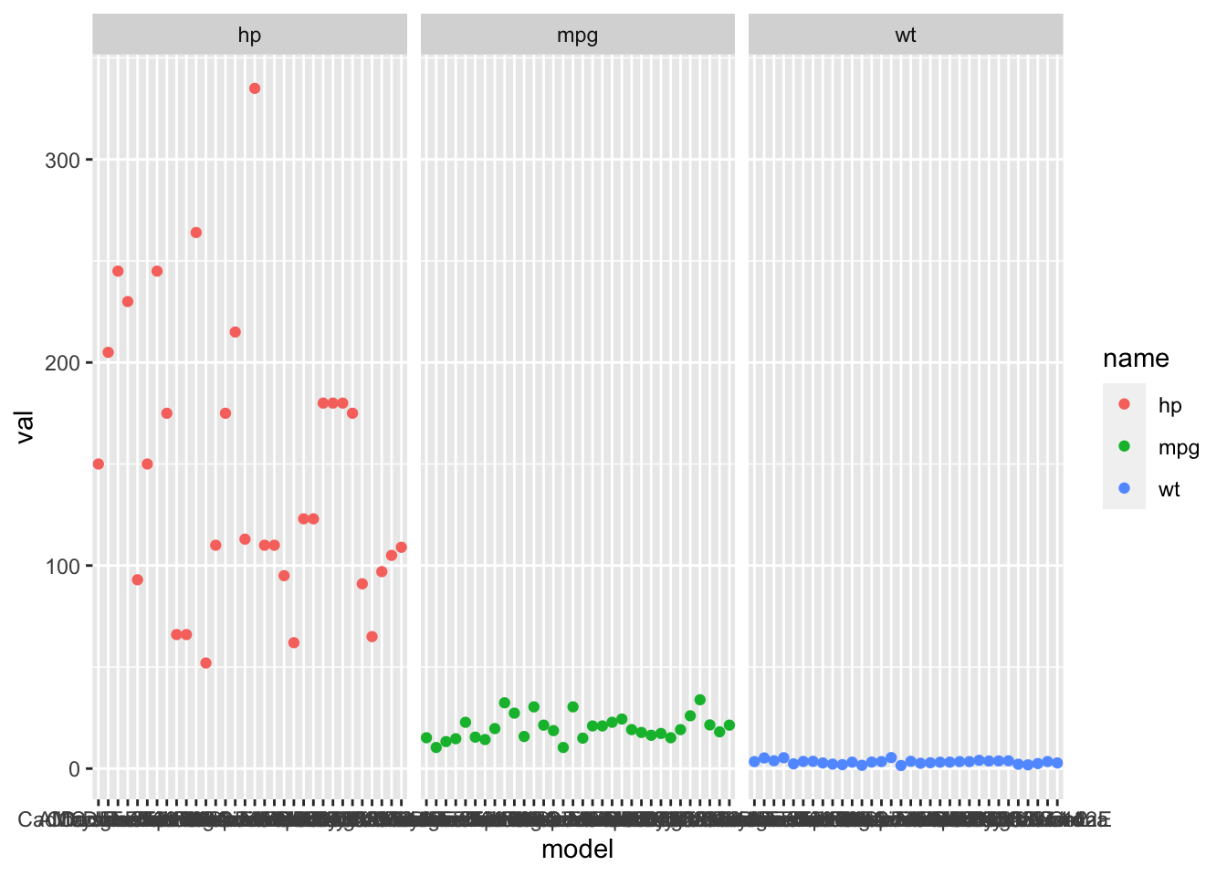

It changed the order our names but that’s ok. We can fix that if needed.

df.long$name <- factor(df.long$name, levels=c("mpg", "wt", "hp"))
ggplot(df.long, aes(x=model, y=val, col=name)) + geom_point() +
  facet_wrap(~name) +
  theme(axis.text.x=element_blank())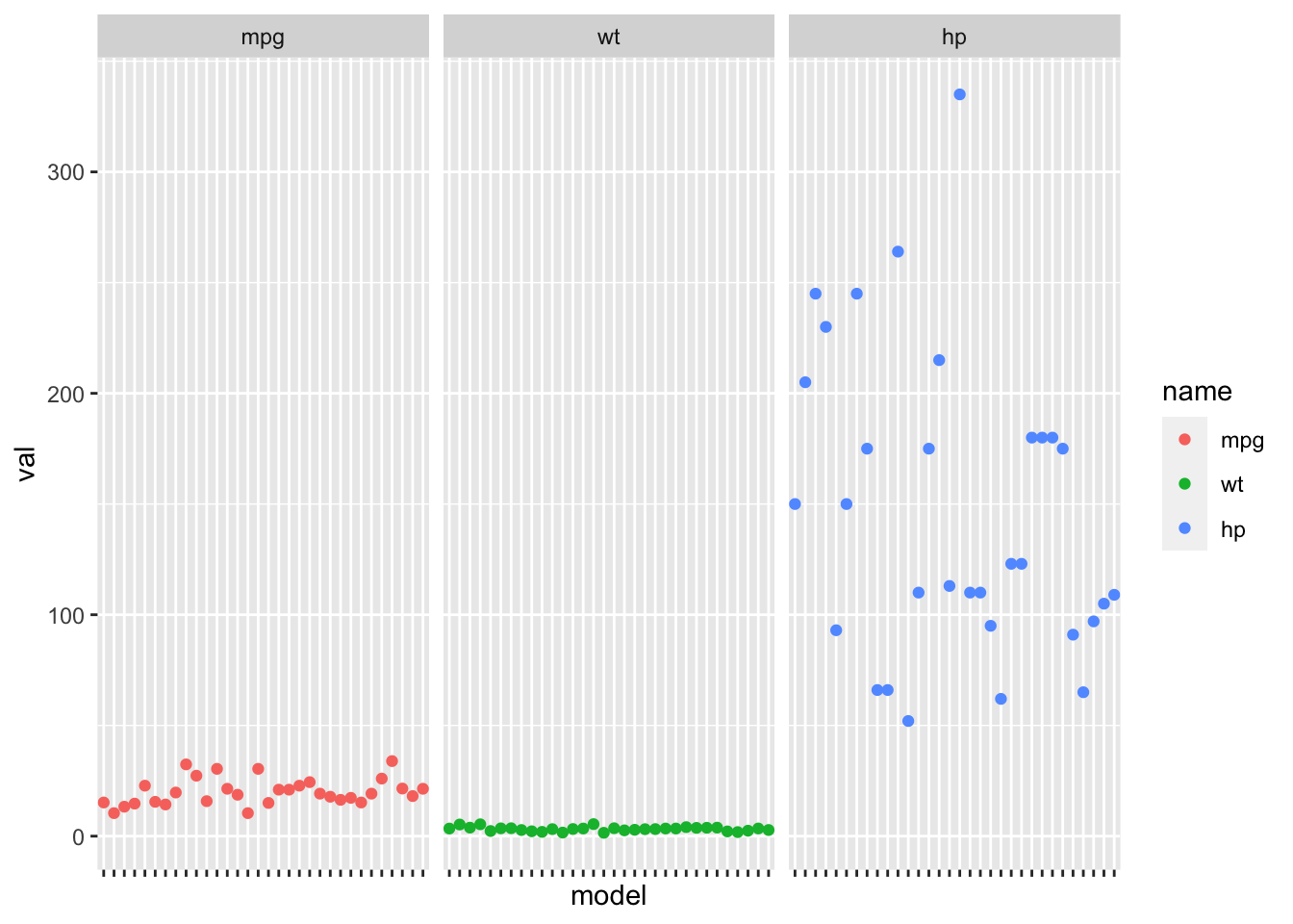

Read ?tidyr::pivot_longer to learn more options but this will be all you need most of the time.

`pivot_wider`

pivot_wider( 
    data frame name,
    names_from = what column has the column names
    values_from = what column has the values
  )

pivot_wider( 
    df.long,
    names_from = "name", 
    values_from = "val"
  )

## # A tibble: 32 x 5
##    model              carb   mpg    wt    hp
##    <chr>             <dbl> <dbl> <dbl> <dbl>
##  1 Mazda RX4             4  21    2.62   110
##  2 Mazda RX4 Wag         4  21    2.88   110
##  3 Datsun 710            1  22.8  2.32    93
##  4 Hornet 4 Drive        1  21.4  3.22   110
##  5 Hornet Sportabout     2  18.7  3.44   175
##  6 Valiant               1  18.1  3.46   105
##  7 Duster 360            4  14.3  3.57   245
##  8 Merc 240D             2  24.4  3.19    62
##  9 Merc 230              2  22.8  3.15    95
## 10 Merc 280              4  19.2  3.44   123
## # … with 22 more rows

BTW, you will normally see the function called with piping.

df.long %>%
  pivot_wider( 
    names_from = "name", 
    values_from = "val"
  )

Comments

I rarely use piping. Why?

Piping is fine but is super slow. Also I develop packages and the R package checks often through errors with piping or any type of implicit reference to data columns in data frames. So like subset(df, x==1) is implicit because it is implying that there is an x column in df but that code will actually work if x is not in df. If you are a package writer, the check will complain about that vagueness.
I have a hard time following long strings of pipes and lose track of what’s going on.

And I rarely use dplyr, tidyr, or tidyverse verbs.

tidyverse is “maturing” which means the functions keep changing…which means my code rots quickly.
I often have to do something that takes me a long time to figure out how to do with tidyverse.

Whereas learning ggplot2 has made my plotting much, much faster, I can’t say the same with data-wrangling with tidyverse except for a few functions that I use to help out with ggplot.

NWFSC Math Bio Program

Week 9: Intro to piping and tidyverse data wrangling