Week 2. More Git + Better Coding Practices
| Compartmentalized | Documented | Extendible | Reproducible | Robust |
Overview
This week I will cover more Git topics and basic coding habits that I have learned over the years. These are good habits that will help make your code less buggy and easier to extend.
Git, GitHub, GitLab
- How to clone someone else’s GitHub or GitLab repository
- How to clone your own repository–when you want to make a copy and use that as a template for something new.
- What are branches, merge conflicts and pull requests?
- Fork or clone? What’s the difference?
- How to add Git to an existing RStudio project and get that on GitHub or GitLab.
Coding Tips
- How to organize and plan your code and why adopting an ‘object-oriented mindset’ will help your code organization (regardless of whether you use object-oriented coding)
- What are namespaces and why you should use
::to call functions. - Tips on writing code and functions in R - little things that will make your code better and more robust
- Tips on things to avoid in your R code, i.e. quirks of R that will tend to create bugs
The material I’m presenting geared toward those who have done a bit of R programming but work mainly with scripts or with functions just for their own use. For new programmers, I recommend The R Student Companion -> R for Data Science -> books specific to your work.
Downloading other people’s repositories
There are two easy ways to do this. Use the one that seems more logical to you.
Method 1.
- In a browser, go to the GitHub (or GitLab) repository you want to copy.
- Copy its url.
- Open GitHub or GitLab.
- If using GitHub, click the
+in top right and clickimport repository. Paste in the url and give your repo a name. - If using GitLab, click
New Projecton right, thenImport Repositorytab, then clickRepo by URL. Paste in url and give repo a name. - Open RStudio and click the project tab in the top right and select,
New Project. Then selectVersion Controland paste in the url of your repository’s url. For example,https://github.com/<youraccount>/Test
- Add the new repo to GitHub Desktop. Open GitHub Desktop, select File>Add Local Repository and navigate to the folder with the new repository.
Method 2.
Steps 1-4 are the same but you can swap step 5 and 6.
- Open GitHub Desktop. Select File>Clone Repository. Paste in the repository url that you are copying and tell it where to save the repository.
- Open RStudio and click the project tab in the top right and select,
New Project. Then selectExisting Directoryand navigate to the directory where you just saved the repo.
You can also clone someone elses repo directly into RStudio or GitHub Desktop and then “Publish” to GitHub or GitLab. I am not going to show that but I show that on this page. For GitLab, it will require issuing Git commands from a terminal. Note, in my experience, method 1 or 2 above is the way to avoid Git-misery as a Git beginner.
Making a copy of your own repository
Let say you want to make a copy of a repository and use it as a template to make something else. And you don’t want the history!
- Make a blank repo on GitHub or GitLab (add that Readme file)
- Pull that down to your computer
- Copy the repo you want to copy into the new repo folder but do not copy the .git folder. Remember the
.gitfolder is hidden.
Code Organization
R is object oriented
Run this code.
fit <- lm(dist ~ speed, data=cars)
class(fit)
## [1] "lm"“lm” is the class of the object “fit”. R knows things to do with objects of class “lm”.
coef(fit)## (Intercept) speed
## -17.579095 3.932409It did that because there is a function coef.lm and R looks for that to see what to do when you pass a “lm” object to coef().
All object of class “lm” are a list with a standard set of items in that list:
names(fit)## [1] "coefficients" "residuals" "effects" "rank"
## [5] "fitted.values" "assign" "qr" "df.residual"
## [9] "xlevels" "call" "terms" "model"That information contains all the information about the fit, the data used for the fit, and the call to lm(). We can just pass fit to print(), plot(), summary(), etc. I could write a new function, foo.lm, to do something new with a “lm” object.
In the call to lm, we had another object, saldat. saldat is class data.frame. lm() knows what to do with data that is a data frame.
Object-oriented mindset
Let’s look at salmon.R. What sort of elements are in this script?
- data
- fits
- predictions
- plots
But the elements are not like “objects”. One data set is a data frame with column headings year, wild, flow, temp and the other is a matrix with years as column headings. The fits are all different types and some have no info about what years or data I fit to (see e.g. fit3). The plots have to be tweaked based on the data and the fits.
Instead we would like to work with “objects” that have a consistent format and have all the information needed for functions that use those objects.
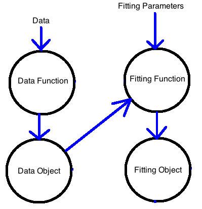
An object
- Has a standardized form (you can describe what elements it needs to have)
- Has all the information that subsequent functions might need to use this object.
- Has information so you know how this object was made
How on earth is one supposed to do this?
…if it is even worthwhile, which I’m not so sure about…
This is part of code organization. Time put into planning and standardizing your code will make you much more efficient (even if it takes time in the beginning) and will definitely help prevent errors and bugs in your code. A big coding project requires this way of thinking.
How do get started
1. Do a little planning on a piece of paper. Example, data:

data planning
2. Then start putting your script in to categories (data, fitting, plotting). Look at salmon.R
3. Write functions instead of long scripts.
Like read_data(), fit_model(), plot1(). This will naturally lead you towards “object-oriented” thinking.
You do not want to be duplicating your code, e.g. lines of code that fit a model or plot, over and over. You’ll just introduce impossible to find errors when you decide to change how you are fitting the data.
Using a few standardized (say plotting) functions will force you to move towards “object-oriented” thinking. So as opposed to copying lines of plotting code over and over when you need a plot like that.
For example, a script:
par(mfrow=c(1,2))
a <- data.frame(year=2000:2009, x=1:10)
plot(a$year, a$x, xlab="year", ylab="count", ylim=c(0,100), xlim=c(1980,2010))

b <- data.frame(YEAR=1980:2009, count=1:30+50)
plot(b$YEAR, b$count, xlab="year", ylab="count", ylim=c(0,100), xlim=c(1980,2010))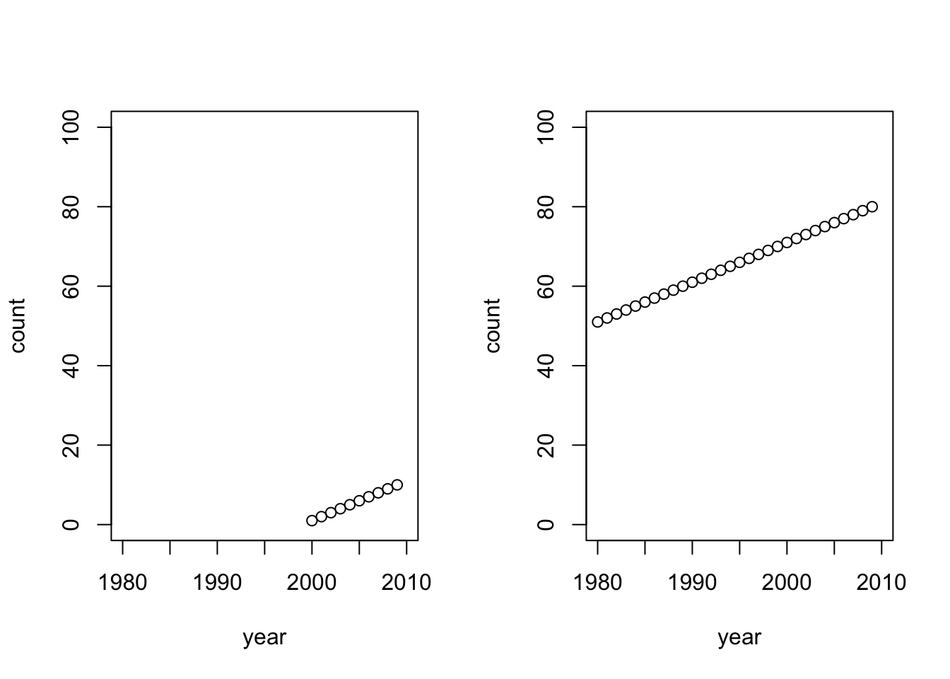
Versus writing a function and standardizing the data frames. This is a toy example.
plot1 <- function(x, xlims=c(1980,2010), ylims=c(0,10)){
  plot(x$year, x$x, xlab="year", ylab="count", ylim=ylims, xlim=xlims)
}

par(mfrow=c(1,2))
a <- data.frame(year=2000:2009, x=1:10)
b <- data.frame(year=1980:2009, x=1:30+50)
ylims <- c(min(a$x,b$x), max(a$x,b$x))
plot1(a, ylims=ylims)
plot1(b, ylims=ylims)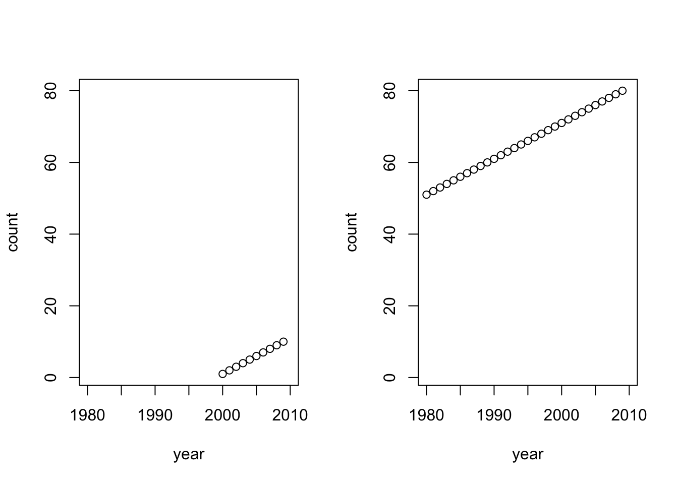
4. Make a plan for your functions
Sketch out the functions that you need to write. You’ll update this as you go along.
5. Have your functions output both the “thing” + the info about that “thing”:
read_data <- function(fil, notes=NULL){
  dat <- read.csv(fil)
  ... bunch of code to fix up the data ...
  if(stringr::str_detect(fil, "Chinook")) species <- "Chinook"
  if(stringr::str_detect(fil, "Coho")) species <- "Coho"

  meta=list(
    file=fil,
    call=deparse( sys.call() ),
    date=Sys.time(),
    notes=notes,
    species=species,
    min.year=min(dat$year),
    max.year=max(dat$year) )

  obj <- list(meta=meta, data=dat)
  return(obj)
}
Next step for object-oriented programming: Weeks 4 and 5 will go into how to assemble your code into an R package and I’ll talk about creating formal objects and methods (like print, plot) for those objects.
Namespaces
- Namespaces. Every function in R belongs to a package. You can be 100% explicit in your function calls by using
::. Soforecast::forecast()would specify theforecastfunction in the forecast package.
Why use this?
- Show in your code what package the function comes from
If you are reading someone else’s code, a great deal of time is lost by not knowing what package a function is from. Where is dismo() from?? If you write dismo::dismo() it is clear it is from the dismo package.
You won’t run into the problem where code fails because you forgot to do
library(package)orrequire(package).You won’t run into problem where you have functions with the same name in two different packages or you accidentally give your function the same name as the function in a package that you need.
This can cause disastrous things to happen to your code when you don’t use Namespaces. Let’s say, unbeknownst to you, someone using your code defines a function called auto.arima().
auto.arima <- function(x){x}Then in your code, you call the auto.arima() function in the forecast package. Because auto.arima() exists in the user’s working directory (global environment), your code fails. auto.arima() should fit a model but it doesn’t since it is overwritten by the user’s function.
library(forecast)## Registered S3 method overwritten by 'quantmod':
## method from
## as.zoo.data.frame zoo##
## Attaching package: 'forecast'## The following object is masked _by_ '.GlobalEnv':
##
## auto.arimaauto.arima(1:10)## [1] 1 2 3 4 5 6 7 8 9 10We have to remove the user’s auto.arima() to get forecast’s function.
rm(auto.arima)
auto.arima(1:10)
## Series: 1:10
## ARIMA(0,1,0) with drift
##
## Coefficients:
## drift
## 1
##
## sigma^2 estimated as 0: log likelihood=Inf
## AIC=-Inf AICc=-Inf BIC=-InfIf we use forecast::auto.arima(), we never run into that problem.
While this may seem rare, when it does happen, it makes a bug that is very hard to track down. Note, for writing packages, use of :: is required.
Various Tips and Quirks of R
- Do not hard code any variables into your scripts or code. Ok. The reality is, you will. Try to hard code less. The more you avoid hard-coding, the faster you will be.
So not this
x <- 1
for(i in 1:10) x <- c(x, 2*i)
but this
n <- 10
w <- 2
x <- 1
for(i in 1:n) x <- c(x, w*i)- Your working directory environment is your enemy (for bugs at least). You will have to keep it clean
rm(list=ls()), use Rmarkdown files to run code (because that uses a clean environment), or assemble your code into an R package.
You can use caching in Rmarkdown files for long runs or save simulation output to Rdata files using save().
All R coders forget this periodically and have wasted significant hours debugging due to a variable left in their environment.
- Use
class()to figure out what R thinks an objects class is. The class of an object determines many things about how R functions respond to an object.
For data.frames, you can use the following code to find out the class of all columns:
a <- data.frame(l = letters, n=1:26)
unlist(lapply(a, class))
## l n
## "character" "integer"Note this does not work because apply is for matrices not data frames.
apply(df, 2, class)## Error in apply(df, 2, class): dim(X) must have a positive length- Data frames are lists not matrices.
Sadly R does not tell you this. And you’ll get errors that can be hard to decipher.
a <- data.frame(a=1:10, b=1:10, c=1:10)
a[,1:2]%*%t(a[,1:2])
## Error in a[, 1:2] %*% t(a[, 1:2]): requires numeric/complex matrix/vector argumentsThe code above doesn’t work because a is not a matrix no matter how much it looks and acts like one.
class(a[,1:2]) # data.frame
class(t(a[,1:2])) # matrix ??
class(a[[1]]) # integer
class(a[1]) # data.frame
class(unlist(a)) # integer- Factors (in data frames) is cause of much trouble. You can avoid with
stringsAsFactors=FALSE
a <- data.frame(a=letters, b=1:26, stringsAsFactors=FALSE)
unlist(lapply(a,class))
## a b
## "character" "integer"Figuring out when you need a character to be a “factor” and when you need it to be a “character” will lead to much suffering, but with time, you’ll figure it out. Remember, class() is your friend.
- R “helps” you bu changing class on your objects…silently. This will cause a frightful number of mysterious bugs and errors.
Example:
a <- data.frame(a=1:10, b=letters[1:10], stringsAsFactors=FALSE)
apply(a, 2, function(x){x[1:2]})
## a b
## [1,] " 1" "a"
## [2,] " 2" "b"What just happened? Why is the a column a character now? apply needs a matrix, so R silently turned your data frame into a matrix. In a matrix all elements need to be the same class. So in this case, R silently changed your numbers to characters. This behavior will also cause mysterious bugs.
Here’s another example. R changes an object of class matrix to class vector.
a <- matrix(1, 3, 3)
apply(a, 2, mean) # this works
apply(a[,1:2], 2, mean) # this works
apply(a[,1], 2, mean) # this throws an error???
## Error in apply(a[, 1], 2, mean): dim(X) must have a positive lengthWhat’s happening is that R dropped the dimensions when you took only one column of a and created a vector. apply will not work on a vector; it is for matrices (or arrays). You can use drop=FALSE to keep the dimensions.
class(a) # matrix
class(a[,1]) #vector
class(a[,1,drop=FALSE]) #matrix- Use
FALSEandTRUEinstead ofFandT
T is a shortcut for TRUE but T is a very commonly used variable name (for time). T is not a protected name but TRUE is. If you use T as a variable name, all your code using T for TRUE will fail.
T=10
T==TRUE
## [1] FALSErm(T)- You can overwrite most any function in R even something like
plot()!!
Say a user writes this function:
plot <- function(x){cat("Yelp!")}Now this plot() function will make all your code with plot() fail. This no longer plots:
plot(1:10)## Yelp!We have to use :: to overcome this:
graphics::plot(1:10)
I’ll remove plot.
rm(plot)While this may seem like it would never happen, it definitely can happen when you share code with other people or use someone else’s code. You can waste hours trying to track down why your code is not working anymore. Use of ::, keeping a clean working environment, use of Rmarkdown files, and use of R packages (that you write) will help protect against this problem.
- Don’t be afraid of using
forloops to get the job done.
You could spend 2-3 hours figuring out how to use tapply() or dplyr to do a task, or just use a for loop.
- Piping means compact code, less memory consumption…. and can be terribly slow computationally. Avoid in simulations.
What’s piping? It’s a function %>% in the magrittr that allows you to string operations together.
library(magrittr)
rnorm(100) %>%
  matrix(ncol = 2) %>%
  apply(2,mean)
## [1] -0.1213327 -0.1913507- Gravitate towards a standard coding style.
Don’t make one up. Use a standard one. I use mainly the tidyverse style guide (or I try). There is a package called styler that has a RStudio plugin that makes it super easy to restyle all your code.
- Gravitate towards a standardized data format.
It’s easier to reuse your plotting functions (and others) if you do that. I use a format similar to tidy data. Try to use the same column headings across projects. Using Brood_Year, year, BROOD_YEAR, and brood.year for brood year across data projects, really slows you down. I see this all the time (and have to fight my own tendency to do this).
- Gravitate towards a standardized names for things you use in your code consistently.
Using alpha, alp, Alpha, a for the same thing in different coding projects makes re-using code much slower.
- Use the here package along with
file.path()to avoid hard-wired directory names.
This will properly construct file paths for whatever operating system you are on. Use the RStudio project feature to get you to the right working directory (that means make sure your project is showing in the top right corner in RStudio).
Instead of this:
setwd('~/GitHub/RWorkflow-NWFSC-2020/data/salmon.R')Use:
fil <- file.path(here::here(), "data", "salmon.R")
fil
That way when you share your code or switch computers, the code doesn’t break.
Week 3
Brief summary of some debugging tools in R and RStudio + mostly RMarkdown.
- debugging functions
- bench-marking
- profiling